This page requires an update, especially to cover wavelets such as CDF 9/7, which is part of the primary lossy (after quantization) compression method for Framework2's native image format. When I get time, I'll do a write-up on the interesting bits.
Bitmaps normally require a lot more storage space as compared to text. Each character on this page is a byte, while an uncompressed bitmap with RGB channels requires 3 bytes per pixel. A 512x512 image at 3 bytes per pixel is 768KB. If we consider that a page of paper holds approximately 2500 characters, then the same space required to store a bitmap of that image could instead hold 314 pages of text. Images are often larger and art resources tend to take up significantly more space than any other type of resources, so it's important to find a good way to compress them.
There are a wide number of ways to hold this information in a lossy compressed form with size, memory and precision tradeoffs. In this article, I will explore image compression with the following topics:
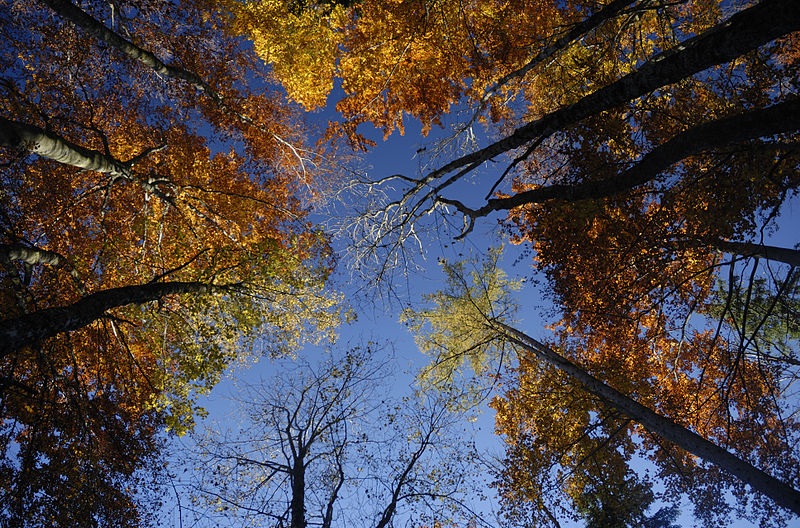 The large amounts of variation in colour and fine details pose a difficult challenge to compress effectively and accurately with lossy compressional algorithms in which detail is lost. At 800x528 with 3 bytes per pixel, this image requires approximately 1237 KB of storage space.
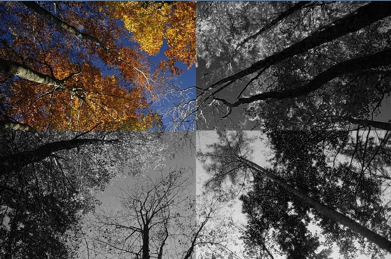
| |
| The channels in the top row are RGB combined and R greyscale. The channels in the bottom row are G greyscale and B greyscale. |
As shown in this image, the image consists of RGB channels. Each of these three channels have high-frequency information that is difficult to compress, contains little redundancy and significantly affects the image quality because the channels are tightly correlated. To decorrelate the channels, a better storage scheme would store luminance and chroma seperately, such as YUV colourspace.
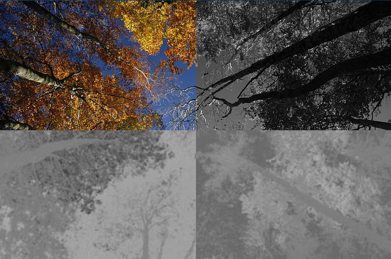 | |
| The channels in the top row are YUV combined and Y (luminance) greyscale. The channels in the bottom row are U greyscale and U greyscale, the chroma channels. |
In this image, you can see that the luminance channel contains the greatest amount of detail while the U and V channels don't have as much variance, allowing them to be downsampled and stored with lower quality without any noticable loss of detail. Downsampling the UV channels to half the original height and width reduce the required bitmap size to 50% of the original required space, given that 2 of the 3 channels now only require 25% of the space that they previously needed. Furthermore, their lower variance makes it easy to compress them with a lossy algorithm because they don't need as much representation as the luminance channel does. If the image wasn't converted to RGB, each of those channels would require as much precision as the luminance channel does.
Conversions between RGB and YUV colourspaces use the following constants:
Wr = 0.299
Wb = 0.114
Wg = 1 - Wr - Wb
Umax = 0.436
Vmax = 0.615
Given RGB values in the range [0,1], YUV is computed as:
	y = Wr * r + Wg * g + Wb * b
	u = Umax * (b - y) / (1 - Wb)
	v = Vmax * (r - y) / (1 - Wr)

	u = (u - -Umax) / (Umax - -Umax)
	v = (v - -Vmax) / (Vmax - -Vmax)
Simplified and optimized:
	y = Wr * r + Wg * g + Wb * b
	u = (-1 - b + Wb + y)/(2Wb - 2)
	v = (-1 - r + Wr + y)/(2Wr - 2)

	y = 0.114b + 0.587g + 0.299r
	u = 0.5 + 0.564334b - 0.564334y
	v = 0.5 + 0.713267r - 0.713267y
Note that while y is in the range [0,1], U and V were computed in the ranges [-Umax,Umax] and [-Vmax,Vmax] respectively, so they are scaled into the range [0,1]. These values may be stored into the YUV channels to represent the image.
To convert back to RGB values, given YUV values in the range [0,1], RGB is computed as:
	u = -Umax + (2 * Umax * u)
	v = -Vmax + (2 * Vmax * v)

	r = y + v * (1 - Wr) / Vmax
	g = y - (u * Wb * (1 - Wb) / (Umax * Wg)) - (v * Wr * (1 - Wr) / (Vmax * Wg))
	b = y + u * (1 - Wb) / Umax
Simplified and optimized:
	r = -1 - 2v(-1 + Wr) + Wr + y
	g = (Wb - 2u*Wb + (-1 + 2)*Wb^2 + Wr - 2v*Wr + (-1 + 2v)*Wr^2 + Wg*y)/Wg
	b = -1 - 2u(-1 + Wb) + Wb + y

	r = -0.701 + 1.402v + y
	g = 0.529136 - 0.344136u - 0.714136v + y
	b = -0.886 + 1.772u + y
Note that u and v are scaled back into the ranges [-Umax,Umax] and [-Vmax,Vmax] respectively. The simplified and optimized versions have scaling included in the transformations, so the values are different from what is normally provided in sample YUV implementations.
When using optimized transform functions that use lower precision values in the conversion process, check that they don't send you a numerically significant amount out of the [0,1] range for either YUV or RGB because when you store the minimum and maximum values present in a channel in a small region of the image, numerical imprecision aggregates after quantization and that region of the image won't be scaled back to its original range. This is especially a problem with the chroma channels where a small block can have very close minimum and maximum values. Even if they only differ by a few bytes (quantize the [0,1] float to a [-128,127] byte), the difference becomes noticable between adjacent blocks on the image. More information on this is in the next sections.
Once chunks are allocated based on the size of quadtree nodes, each chunk represents a waveform to be used with the following sections, transform and quantization. For processing, the precision of the waveform's values needs to be higher than the 1-byte representation per value that it's currently at. The next step is to transform this waveform into something with more redundancy. The quality of the compressed image will dependant on the accuracy of the compressed transformed waveform versus the uncompressed transformed waveform. The memory required to store the compressed waveform will be dependant on how little memory this waveform will be reconstructed from.
The aim of this transform is to convert the waveforms in each chunk to a frequency domain representation. The inverse of this transform can convert a frequency domain waveform back to an amplitude-based domain. A Discrete Fourier Transform is suited to this, but it works on complex numbers with real and imaginary parts. Since a transform neither adds nor removes points, we shouldn't double the size of our points (real -> real + imaginary), so the cut-down Discrete Cosine Transform is ideally suited for this task. In this situation, we use a 2D DCT on the 2D chunks of each channel instead of a 1D DCT on a linear waveform. The DCT coefficients required to represent this waveform are computed by:
	c[i, j] = Sum(x,0,xw) Sum(y,0,yw) w[x,y] * cos[(pi/8)(x + 1/2)(u)] * cos[(pi/8)(y + 1/2)v]

	xw = horizontal width
	yw = vertical width
	w[x,y] = Waveform amplitude at x,y in the chunk
	u = horizontal spatial frequency for 0 <= u <= xw
	v = vertical spatial frequency for 0 <= v <= yw
There are different implementations of the formal definition of DCT. The ones used here, specifically, are DCT-II for the forward transform and DCT-IV for the inverse transform. The DCT stores a DC component in the first element of the transformed waveform, followed by the rest of the coefficients which are called AC components. A nice benefit of the DCT is that the AC components towards the top-left of the transformed matrix have more significant values, this will be explored further during quantization.
A wavelet transform is a different type of transform, one that won't be easily used in lossy compression. It relies on redundancy and won't have any effect on anything statistically comparable to random noise. First, you take the entire waveform (each channel of the image) and split it into chunks of 4. The first value of each chunks, unmodified, will be copied to position n where n is the chunk number. The difference between the first chunk and each of the other 3 chunks will be stored in the other 3 quarters of the waveform. This process is repeated a few times for the first quarter of the waveform until it's at a small size where precisiom would make reconstruction difficult. The aim is to get similar deltas and redundancy grouped together for lossless compression. Lossy compression at any level, will make reconstruction extremely inaccurate, particularily at higher levels.
The sections below are commonly available, so I won't write about them in much detail here.